Table of Contents Show

Rate this post

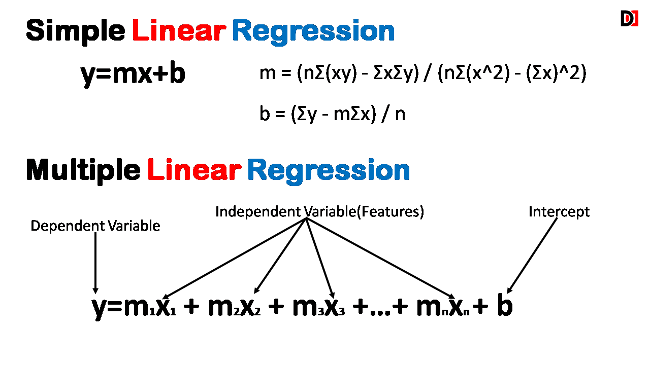
Multiple Linear Regression is an extension of Simple Linear Regression. While Simple Linear Regression models the relationship between one independent variable and one dependent variable, Multiple Linear Regression considers the influence of multiple independent variables on a single dependent variable.

Key Concepts

1. Multiple Independent Variables: Instead of a single predictor, we now have multiple factors influencing the dependent variable.

Example: Predicting house prices based on size, age, number of bedrooms, location, etc.

2. Dependent Variable: Remains the same – the variable we are trying to predict.

3. Linear Relationship: The model assumes a linear relationship between the dependent variable and the combined effect of the independent variables.

Mathematical Representation

The equation for Multiple Linear Regression is:

y = b0 + b1x1 + b2x2 + ... + bn*xn

where:

y: The predicted value of the dependent variable.
x1, x2, …, xn: The values of the independent variables.
b0: The intercept (the value of y when all independent variables are 0).
b1, b2, …, bn: The coefficients representing the influence of each independent variable on the dependent variable.

Multiple Linear Regression vs Simple Linear Regression:

Finding the Best-Fit Hyperplane

In Multiple Linear Regression, we are essentially trying to find the best-fitting hyperplane (a multi-dimensional plane) that minimizes the difference between the actual values of the dependent variable and the predicted values.

Example: Predicting House Prices

Let’s say we want to predict house prices based on size (square footage), age, and number of bedrooms. We have the following data:

Size (sq ft)	Age (years)	Bedrooms	Price (in thousands)
1500	10	3	250
2000	5	4	300
1800	8	3	280
1200	20	2	180
2500	2	5	400

Using scikit-learn in Python:

Import necessary libraries:

import numpy as np
from sklearn.linear_model import LinearRegression

Prepare the data:

X = np.array([[1500, 10, 3], 
             [2000, 5, 4],
             [1800, 8, 3],
             [1200, 20, 2],
             [2500, 2, 5]])  # Independent variables
y = np.array([250, 300, 280, 180, 400])  # Dependent variable (house price)

Create and train the model:

model = LinearRegression()
model.fit(X, y)

Make predictions:

new_house = np.array([[1850, 12, 4]])  # New data point
predicted_price = model.predict(new_house)
print("Predicted Price:", predicted_price)

This will give you the predicted price of a house with the given characteristics.

Applications of Multiple Linear Regression:

Predicting customer churn
Forecasting sales based on various factors
Analyzing the impact of multiple factors on health outcomes
Developing credit risk models

Limitations

Assumes a linear relationship between the dependent variable and the independent variables.
Sensitive to outliers and multicollinearity (high correlation between independent variables).
May not capture complex non-linear relationships.

Multiple Linear Regression is a powerful technique for modeling the relationship between a dependent variable and multiple independent variables. By understanding its principles and limitations, you can effectively apply this method to various real-world problems.

< Previous

Next >