Machine Learning models are designed to learn patterns from data and make predictions or decisions. However, in the quest for better accuracy, they can sometimes learn noise or irrelevant details, leading to overfitting. Regularization is a vital concept in machine learning that helps address this problem, ensuring the models generalize well to unseen data.

In this article, we will explore regularization in detail, covering its importance, techniques, and how it can be implemented effectively. Let’s dive in

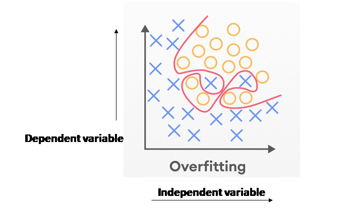
Overfitting is a common challenge in machine learning, where a model performs exceptionally well on the training data but poorly on new, unseen data. This happens because the model has learned the noise and intricacies of the training data too well, failing to generalize to real-world scenarios. Regularization is a powerful technique designed to address this issue.

What is Regularization?

Regularization is a technique used to prevent overfitting by adding a penalty term to the model’s loss function. This penalty discourages the model from becoming overly complex and helps it focus on the most critical patterns in the data.

By controlling the model’s complexity, regularization ensures that it performs well on both the training data and new, unseen data. It effectively balances the trade-off between bias and variance, improving the model’s ability to generalize.

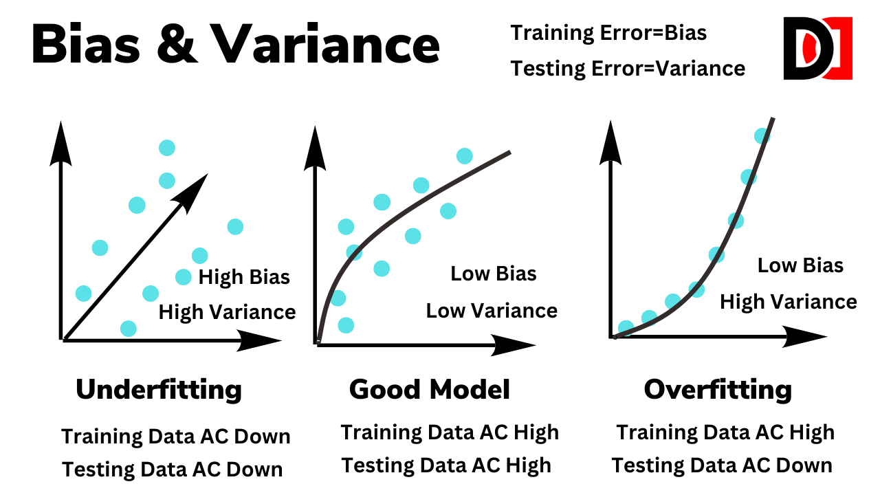
What are Bias and Variance?

Click here to read the complete guide about bias and variance.

Why is Regularization Important?

• Prevents Overfitting: Regularization reduces the risk of overfitting by penalizing overly complex models.
• Enhances Generalization: It helps the model perform better on unseen data, avoiding high variance.
• Simplifies Models: By constraining coefficients or parameters, regularization leads to simpler, more interpretable models.
• Handles Multicollinearity: Regularization can deal with multicollinearity in datasets, especially in regression problems, by shrinking coefficients.

Types of Regularization Techniques

1. L1 Regularization (Lasso)

L1 regularization adds the absolute value of the coefficients as a penalty term to the loss function. It is defined as:

• Key Features:
  • Performs feature selection by shrinking some coefficients to exactly zero.
  • Useful when you suspect many features are irrelevant.
• Applications:
  • Sparse data problems, feature selection in regression.
• Mathematical Representation:
  • L(β)=Loss Function+λ∑∣βi​∣.

2. L2 Regularization (Ridge)

L2 regularization adds the square of the coefficients as a penalty term to the loss function. It is defined as:

• Key Features:
  • Shrinks coefficients but does not set them to zero.
  • Prevents large coefficients, reducing multicollinearity.
• Applications:L2 Regularization (Ridge)
  • Regression problems where all features are important.
• Mathematical Representation:
  • L(β)=Loss Function+λ∑βi2​​.

3. Elastic Net

Elastic Net combines L1 and L2 regularization, adding both absolute and squared penalties:

• Key Features:
  • Handles both feature selection and multicollinearity.
  • Provides a balance between Lasso and Ridge.
• Applications:
  • High-dimensional data where features may be correlated.
• Mathematical Representation:
  • L(β)=Loss Function+λ1​∑∣βi​∣+λ2​∑βi2​.

4. Dropout Regularization

Dropout is a regularization technique specifically for neural networks. It randomly “drops out” or ignores certain neurons during training, preventing co-dependencies among neurons.

• Key Features:
  • Reduces overfitting in deep learning models.
  • Makes the model robust by introducing randomness.
• Applications:
  • Deep neural networks for classification or regression tasks.

5. Early Stopping

Early stopping is a simple and effective regularization technique. It involves monitoring the model’s performance on a validation set and halting training when the performance stops improving.

• Key Features:
  • Prevents over-training on the dataset.
  • Requires a separate validation set.
• Applications:
  • Any model trained iteratively, such as neural networks or gradient boosting.

6. Data Augmentation

Data augmentation increases the diversity of the training data by applying transformations, such as rotations, translations, and noise.

• Key Features:
  • Reduces overfitting by making the model robust to variations.
  • Does not explicitly modify the loss function.
• Applications:
  • Image recognition, natural language processing, and other domains with limited data.

7. Weight Constraints

Weight constraints limit the magnitude of weights during training. Examples include max norm constraints and unit norm constraints.

• Key Features:
  • Prevents weights from growing too large.
  • Useful in neural networks.
• Applications:
  • Models prone to exploding gradients.

8. Batch Normalization

Batch normalization normalizes input features for each batch during training. While not explicitly a regularization technique, it has a regularizing effect by reducing internal covariate shift.

• Key Features:
  • Improves convergence.
  • Regularizes models with deeper architectures.
• Applications:
  • Deep learning, especially convolutional and recurrent neural networks.

9. Noise Regularization

Adding noise to inputs, weights, or activations during training can act as a form of regularization.

• Key Features:
  • Encourages the model to learn robust features.
  • Simulates data variability.
• Applications:
  • Neural networks, especially for time-series or image data.

Comparison of Ridge, Lasso, and Elastic Net

Aspect	Ridge	Lasso	Elastic Net
Penalty Type	L2	L1	L1 + L2
Feature Selection	No	Yes	Yes
Multicollinearity	Handles Well	Struggles	Handles Well
Coefficients	Shrinks	Some to Zero	Combination

What are Overfitting and Underfitting?

Click here to read the complete guide about Overfitting and Underfitting.

Choosing the Right Regularization Technique

The choice of regularization technique depends on the model, dataset, and problem:

• Use L1 or Elastic Net for feature selection.
• Use L2 for ridge regression and to handle multicollinearity.
• Use Dropout or Batch Normalization for neural networks.
• Apply Data Augmentation for image or text data with limited examples.
• Use Early Stopping for iterative models with a validation set.

Practical Implementation of Regularization

Here are examples of implementing regularization in Python:

L1 and L2 Regularization in Scikit-learn:

from sklearn.linear_model import Lasso, Ridge

# Lasso (L1 Regularization)
lasso = Lasso(alpha=0.1)
lasso.fit(X_train, y_train)

# Ridge (L2 Regularization)
ridge = Ridge(alpha=1.0)
ridge.fit(X_train, y_train)

Dropout in TensorFlow:

from tensorflow.keras.layers import Dropout

model.add(Dense(128, activation='relu'))
model.add(Dropout(0.5))  # Dropout rate of 50%

Early Stopping in TensorFlow:

from tensorflow.keras.callbacks import EarlyStopping

early_stopping = EarlyStopping(monitor='val_loss', patience=5)
model.fit(X_train, y_train, validation_data=(X_val, y_val), callbacks=[early_stopping])

Regularization is a cornerstone of building robust and generalizable machine learning models. By penalizing complexity, it ensures that models focus on meaningful patterns in the data and avoid overfitting. Whether you’re working with simple regression or complex neural networks, understanding and applying regularization techniques is essential for achieving optimal performance.